In production environments, early detection is the difference between smooth operations and a crisis. Traditional monitoring systems fail in three critical ways: they do not correlate anomalies across infrastructure layers, they alert on symptoms rather than root causes, and they provide no predictive intelligence. This article describes an offline anomaly detection and reliability intelligence engine that solves all three problems.
The Problem
Traditional monitoring systems suffer from three critical gaps:
Blind Spots Across Layers: When query latency spikes, operators do not know if the root cause is disk I/O, CPU saturation, or memory pressure. Anomalies are detected in isolation without cross-layer correlation.
Reactive Alerting: Systems alert after problems begin affecting users. Operators spend 30 minutes investigating root causes while service degrades.
No Predictive Intelligence: Disk exhaustion, connection saturation, and replication lag arrive as surprises. By the time they become critical, remediation is impossible.
Additionally, in offline environments (regulated industries, air-gapped networks), external machine learning services are unavailable. Organizations must rely entirely on local intelligence.
The Solution
The system implements three phases that progressively add intelligence:
Phase 1: Cross-Layer Metrics Collection
Every five minutes (configurable), the system collects 50+ metrics from five infrastructure layers:
Pgpool: Connection pool utilization, failover events, routing errors, node health
Storage: Disk I/O latency, queue depth, IOPS, disk space usage, growth rate
Operating System: CPU usage, memory usage, load average, process count, file descriptors
Network: Throughput, packet loss, latency
The system retains 30 days of historical data (8,640 data points per metric), creating a foundation for machine learning.
Phase 2: Anomaly Detection and Root-Cause Intelligence
When an anomaly is detected, the system performs a four-step analysis:
Detection: The system identifies anomalies using four parallel methods: statistical deviation (Z-score), percentile-based detection (95th percentile), rate of change detection (acceleration), and Isolation Forest (multivariate patterns).
Correlation Analysis: The system examines all other metrics to find correlations. If query latency is high, it checks disk I/O, CPU, memory, and connection pool simultaneously.
Root Cause Ranking: The system ranks potential causes by correlation strength. A correlation of 0.91 between disk I/O and query latency is strong evidence. A correlation of 0.42 is weak evidence.
Confidence Scoring: The system calculates confidence (0-1 scale), combining anomaly severity, correlation strength, and model fit quality. High confidence (>0.85) warrants immediate action.
e.g.: Query latency spikes to 2,500 ms (baseline 500ms)
The system detects this as a 92/100 anomaly. It finds that disk I/O latency is also high (correlation 0.91), CPU is elevated (correlation 0.65), and the connection pool is slightly high (correlation 0.42). It ranks disk I/O as the root cause with 92% confidence. Overall confidence is 0.87.
The operator receives a read-only investigation alert with ranked root causes, evidence trails, and safe investigation steps. The operator identifies the root cause in 2 minutes instead of 30.
Phase 3: Predictive Risk Forecasting
The system implements five machine learning models that forecast operational failures:
Disk Exhaustion Prediction: Uses linear regression on disk growth trends. Accuracy 92%. Example: Current 80% capacity, growing 1 GB/day = 12 days to critical.
Connection Saturation Prediction: Forecasts days until max connections. Accuracy: 88%. Example: 380/500 connections, growing 3.2/day = 45 days to saturation.
Replication Lag Prediction: Calculates the probability of lag exceeding the threshold. Accuracy 85%. Example: 25s lag, 60s threshold, growing 2.5s/day = 14 days to breach.
The system implements continuous learning without external dependencies:
Incremental Model Updates: Models retrain every 15 minutes using 42 data points (7 days). Completes in milliseconds.
Adaptive Baselines: The system learns what normal looks like for each metric. Query latency baseline at 9 AM Monday differs from 2 AM Sunday.
Anomaly Fingerprinting: The system learns patterns of known issues (backup spikes, autovacuum CPU). Suppresses false positives.
Correlation Learning: The system learns which metrics correlate. Disk I/O leads to query latency by 5 minutes.
Confidence Scoring: Every prediction includes confidence, combining anomaly score, correlation strength, and model fit quality.
key Features
Offline-First: All intelligence is generated locally. No internet, no cloud services, no external APIs.
Cross-Layer Correlation: Detects root causes versus symptoms. Ranks hypotheses by confidence.
Predictive Intelligence: Forecasts disk exhaustion, connection saturation, replication lag, query regression, and Pgpool instability.
Safe Operator Guidance: Read-only investigation steps only. No destructive actions. Human operators maintain accountability.
Continuous Learning: Models adapt automatically to changing infrastructure behavior.
Real-world Impact
Traditional System: Alert fires → Operator investigates 30 minutes → Root cause identified → Service degraded
Intelligent System: Alert fires with root cause analysis → Operator identifies cause in 2 minutes → Service protected
Time saved: 28 minutes of investigation plus 12 days of advance notice for planning.
Conclusion
This offline anomaly detection engine transforms PostgreSQL monitoring from reactive to proactive. By correlating metrics across infrastructure layers, calculating confidence scores, and forecasting failures, operators detect issues faster, understand root causes, predict failures days in advance, and operate safely with read-only guidance.
The system works in fully offline environments. Statistical analysis and intelligent correlation replace expensive machine learning infrastructure while providing superior operational insights.
In the current landscape of generative AI, organizations are grappling with a core limitation of large language models (LLMs): they only know what they have been trained on and lack access to proprietary or real-time enterprise data. To bridge this gap, Retrieval Augmented Generation (RAG) has become the dominant architecture, and PostgreSQL, equipped with the pgvector extension, is emerging as the industry’s “Swiss Army knife” for managing the high-dimensional data that powers these systems.
Why pgvector is a Game Changer
The traditional approach to AI search involved moving data into specialized, standalone vector databases. However, pgvector allows you to store vector embeddings directly alongside your existing relational data. This provides data proximity, which reduces the steps needed to return information to the user and allows you to leverage a rich, battle-tested tooling ecosystem of client drivers and ORMs.
Instead of searching for exact keyword matches, vector search tries to understand the semantic meaning or context of a query. By converting text, images, or audio into numerical vectors, machines can quantify similarity using metrics like Euclidean (L2), cosine, or inner product distance.
Choosing Your Strategy: HNSW vs. IVF_FLAT
To search through millions or billions of vectors efficiently, indexing is mandatory. PostgreSQL offers two primary paths:
• IVF_FLAT: This method chunks vectors into lists using a K-means algorithm to find centers. It is very fast to build but may require visiting more lists to maintain high recall (accuracy), which can degrade performance.
• HNSW (Hierarchical Navigable Small Worlds): Recognized as the state-of-the-art indexing method, HNSW creates a layered graph of connections between similar vectors. It provides superior performance and recall without the trade-offs of IVF_FLAT and is particularly well-suited for data sets where vectors are continuously added.
The RAG Lifecycle in PostgreSQL
Implementing a high-performance AI application within PostgreSQL follows a straightforward pipeline:
1. Data Ingestion: Ingest unstructured data like PDFs or CSVs and use specialized loaders to convert them into a structured format.
2. Embedding Generation: Pass this data through a model (like OpenAI’s text-embedding-3 or Amazon Bedrock’s Titan) to generate a vector, typically between 1,536 and 4,000 dimensions.
3. Vector Storage: Save the vector in a table with the vector data type.
4. Retrieval: When a user asks a question, convert that query into an embedding and perform a similarity search in the database using the ORDER BY clause and a distance operator.
5. Generation: Provide the retrieved context to the LLM to generate a response that is grounded in factual, proprietary information, thereby minimizing hallucinations.
Scaling to the Terabyte Era
PostgreSQL is built for scale, supporting a maximum table size of 32 Terabytes (TB). However, high-velocity AI workloads require careful management of Transaction ID (TXID) Wraparound to prevent catastrophic failures where data becomes “invisible.” Experts recommend declarative partitioning once tables exceed 100GB to allow for parallel vacuuming and maintenance, ensuring the database remains healthy even as AI data grows exponentially.
That’s said
Open-source innovation moves fast. With the ability to build conversational agents that possess long-term memory via pgvector, developers no longer have to choose between the reliability of a relational database and the power of a vector store. By integrating these capabilities into a single environment, you can future-proof your applications while maintaining the durability and crash recovery standards that have made PostgreSQL a leader since its inception in 1986.
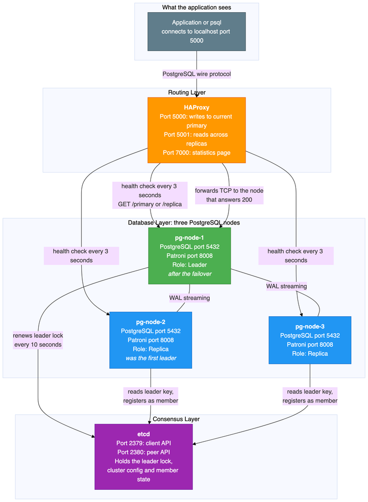
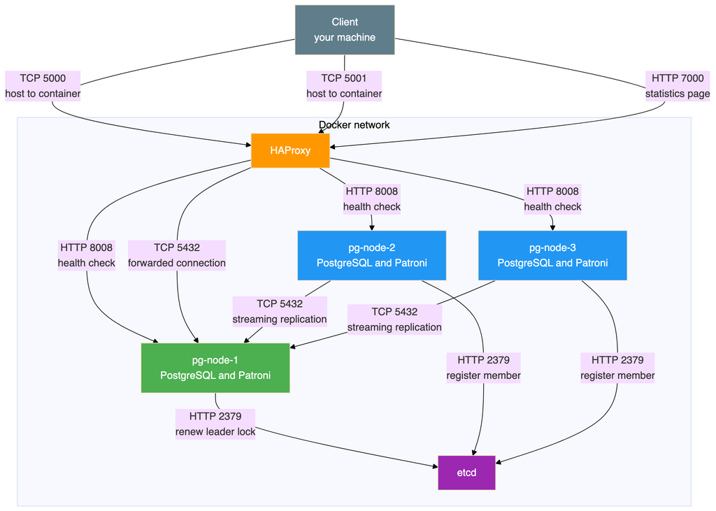
The cluster has three PostgreSQL nodes managed by Patroni, one etcd node holding the leader lock, and HAProxy giving the application one address to connect to. Everything runs in Docker on a single machine.
Every timestamp, log line, WAL position and row count in this document comes from a real test run. Nothing has been made up or filled in for illustration. Where a number is specific to this environment, the text says so.
The environment is built from four components, each with one job.
PostgreSQL 16.4 is the database engine. It stores the data, runs the queries, and ships its write ahead log to the replicas.
Patroni 3.3.2 is the high availability manager. It runs next to PostgreSQL on every node and decides which node is the primary. It starts PostgreSQL, promotes it, demotes it, and rebuilds replicas when needed.
etcd 3.5.15 is the distributed configuration store. Patroni keeps the leader lock and the cluster state there.
HAProxy 2.9 is the connection router. It gives clients one stable address and sends them to whichever node is currently the primary.
Everything runs under Docker Compose on a single Docker host.
The captured HAProxy log has no timestamps, because HAProxy writes these particular messages without them. The order of events and the exact reason codes are therefore verified, but the few seconds attributed to HAProxy noticing the change are derived from the configured three second check interval rather than measured.
The moment the primary container was stopped, given below as 14:51:58, comes from the command output at the time. It is the one figure in the failover timeline that is not in a log file. Everything after it is.
The failover script in the repository writes a marker row whose text ends with a timestamp, but the captured row has no timestamp in it. The recovery script writes a marker row of its own, and no such row exists in the captured table at all. The row that does exist for the replica test is not written by any script in the repository. On top of that, the state capture script writes sixteen files per snapshot, while the committed snapshots contain ten, one of which no script produces.
The conclusion is that the scripts were revised after this run. The captured output is genuine, and it agrees with itself everywhere it can be cross checked. What cannot be claimed is that running these scripts today produces exactly the files shown here.
Which component solves which problem, and which problems each component does not solve.
Why the leader lock is kept in etcd rather than inside PostgreSQL.
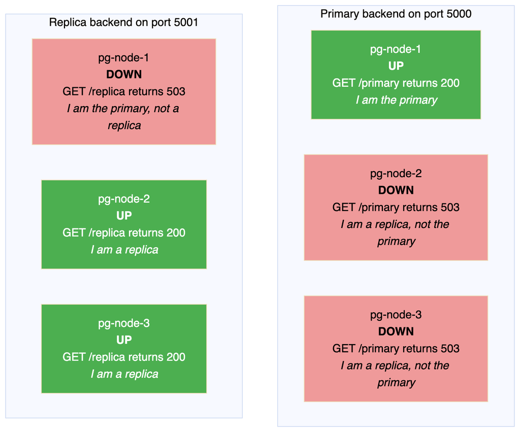
Why a healthy HAProxy dashboard is supposed to show some servers as DOWN.
What happens to connections that are already open when a failover starts. The honest answer catches people out.
When a failed primary needs pg_rewind to rejoin, and when it does not. In this run it did not, which is the more common case than the write ups suggest.
Anyone who runs PostgreSQL and has been asked what happens if the database goes down. You need to be comfortable with Docker, a terminal and basic SQL. No previous Patroni experience is needed.
An important limit on scope
This is a laboratory build. Five containers on one Docker host, with a single etcd node, is a good way to learn the mechanics.
This architecture removes that single point of failure. Several copies of the database stay in step with each other. If the primary stops, one of the copies takes over on its own, with no manual work and no change to the connection string on the application side.
There are four separate problems to solve here:
Keeping more than one copy of the data. This is done by PostgreSQL streaming replication.
Noticing that the primary has died, and choosing a replacement. This is done by Patroni together with etcd.
Actually promoting the chosen replica. This is done by Patroni.
Sending application traffic to whichever node is currently the primary. This is done by HAProxy.
Each component handles one of these. There is no overlap, which is useful when something breaks, because the split tells you where to look.
PostgreSQL is the database itself: tables, indexes, data, SQL processing, transactions and constraints. It runs on all three nodes, but only one node accepts writes at any moment. The other two are read only replicas.
What PostgreSQL does here:
Stores the application data.
Processes SQL from the application.
Maintains the write ahead log, which is a sequential record of every change made to the database.
Sends those log records to the replicas over streaming replication. This is how the replicas keep up.
On a replica, replays incoming log records so the same changes are applied locally.
Runs replicas in hot standby mode, which means they can answer read only queries while they are still receiving replication data.
What PostgreSQL does not do:
It does not decide which node is the primary. It has no idea that a cluster exists.
It does not fail over. If the primary dies, PostgreSQL on a replica simply waits for more log data. It will not promote itself.
It does not route connections. It listens on port 5432 and serves whatever connects.
Port
Protocol
Purpose
5432
PostgreSQL wire protocol over TCP
Database connections
Some PostgreSQL terms that appear throughout this document:
Write ahead log, usually shortened to WAL in the tools themselves. Every insert, update, delete and schema change is written to this log before it is applied to the data files. Replication is built on top of it, because a replica receives and replays exactly the same records.
Timeline. A counter that increases by one every time a replica is promoted. Timeline 1 is the original primary. Timeline 2 means one promotion has happened. This test moved from timeline 1 to timeline 2.
Log sequence number. A position in the log stream. Comparing the sent, written, flushed and replayed positions between primary and replica tells you how far behind a replica is.
The pg_is_in_recovery function. Returns true on a replica and false on the primary. This is how you check a node’s role from SQL.
The pg_stat_replication view. A view on the primary that lists every connected replica, its state, and how far behind it is.
The pg_rewind tool. Rewinds a former primary’s data directory back to the point before it diverged from the current primary. This lets a failed primary rejoin as a replica without copying the entire database again.
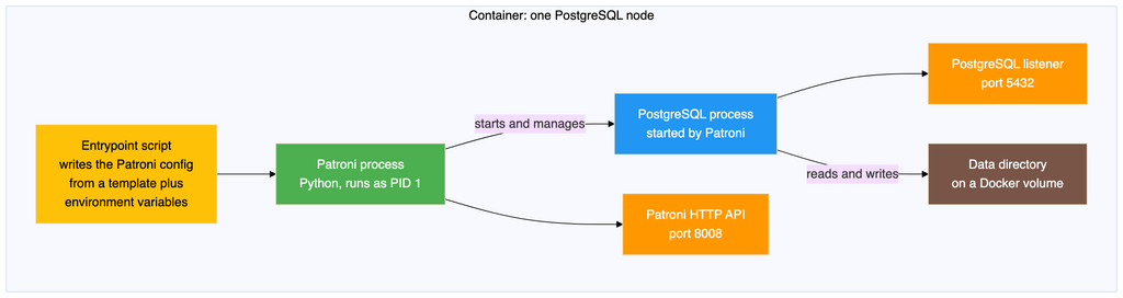
Patroni is a Python program that runs next to PostgreSQL on every node. It stores no data and runs no SQL of its own. Its job is to manage the PostgreSQL instance and to coordinate with the other nodes through etcd.
What Patroni does:
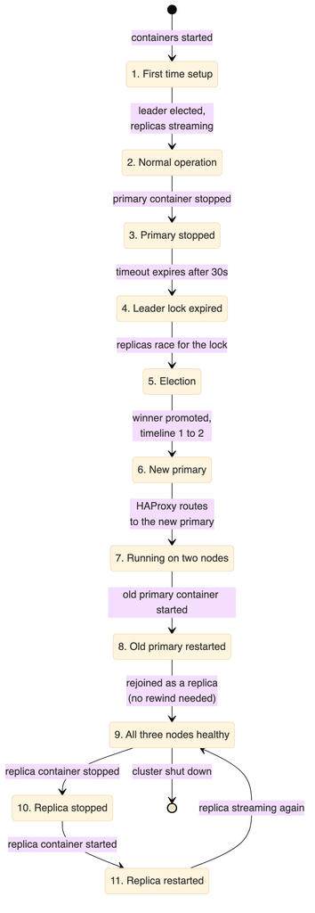
First time setup. When the cluster starts for the first time, one Patroni instance wins a lock in etcd and creates the PostgreSQL data directory. The other instances see that a leader already exists, copy the leader’s data with a base backup, and start PostgreSQL as replicas.
Leader lock management. The current leader has to renew its lock in etcd every ten seconds. If it fails to renew before the thirty second timeout expires, the lock becomes available to the other nodes.
Health monitoring. Patroni watches the local PostgreSQL process. If PostgreSQL stops, Patroni tries to restart it. If it cannot, Patroni gives up the leader lock.
Election and promotion. When the leader lock expires, the surviving Patroni instances race to take it. The winner promotes its local PostgreSQL from replica to primary.
Demotion and recovery. When a former primary comes back, Patroni sees that another node holds the lock. It runs pg_rewind to bring the local data directory back in line, then starts PostgreSQL as a replica of the new leader.
A small HTTP API. Patroni answers on port 8008 and reports the node’s current role. HAProxy uses this for health checks.
Configuration management. Patroni writes the PostgreSQL configuration files, the host based authentication file, and the standby signal files. You do not edit those by hand, because Patroni will overwrite them.
What Patroni does not do:
It does not store application data. It is a management process, not a database.
It does not route client connections. Applications never connect to Patroni.
It does not provide the consensus itself. It relies on etcd for that.
Port
Protocol
Purpose
8008
HTTP
Health check endpoint for HAProxy, and cluster status queries
The API endpoints that matter in this build:
Endpoint
Returns 200 when
Returns 503 when
Used by
GET /primary
This node is the primary
This node is a replica
The HAProxy primary backend
GET /replica
This node is a replica
This node is the primary
The HAProxy replica backend
GET /health
PostgreSQL is running and healthy
PostgreSQL is down
The Docker health check
GET /patroni
Always, returning full node state
Not applicable
Diagnostics
The Patroni settings used here:
Setting
Value
What it means
scope
pg-ha-cluster
The cluster name. Every Patroni instance with the same scope belongs to the same cluster.
name
pg-node-1, pg-node-2, pg-node-3
A unique name for each node. It must differ on every node.
namespace
/service/
The key prefix Patroni uses inside etcd.
ttl
30 seconds
How long the leader lock stays valid. If the leader does not renew inside this window, the lock expires and other nodes may take it.
loop_wait
10 seconds
How often the Patroni main loop runs. Each pass checks PostgreSQL, renews the lock if this node is the leader, and looks for changes in etcd.
retry_timeout
10 seconds
How long Patroni keeps retrying etcd and PostgreSQL operations before giving up.
maximum_lag_on_failover
1048576 bytes, which is 1 MB
A replica must be within this many bytes of the primary to be allowed to take over. This stops a badly lagging replica from being promoted and losing data.
use_pg_rewind
True
When a former primary rejoins, use pg_rewind instead of a full base backup. Recovery is far faster.
use_slots
True
Use replication slots, so the primary does not throw away log segments that a replica still needs.
etcd is a key value store with strong consistency guarantees. In this build it answers one question that matters more than any other: which node is the leader?
Patroni nodes do not talk to each other to elect a leader. They all talk to etcd instead. etcd guarantees that only one node can hold the leader lock at a time, because creating the key is an atomic operation.
What Patroni keeps in etcd, under the key prefix for this cluster:
Key
Content
Purpose
leader
The name of the current leader
The leader lock. Whichever node created this key is the primary. It expires after the timeout.
initialize
A cluster initialisation token
Stops two nodes from creating a data directory at the same time during first startup.
config
Cluster wide PostgreSQL configuration
Shared settings, so all nodes agree.
members/pg-node-1
Connection details, state, timeline and log position for that node
Each node registers itself so the others know how to reach it.
members/pg-node-2
The same, for node 2
members/pg-node-3
The same, for node 3
How the leader lock actually works:
A Patroni node starts and checks etcd for an existing leader key.
If there is no leader key, or the old one has expired, the node tries to create one with its own name and a thirty second lifetime.
etcd allows only one of those creates to succeed. The node that wins becomes the leader.
The leader has to renew the key before it expires. It renews every ten seconds, so it gets three attempts inside the thirty second window.
If the leader stops renewing, because it crashed or lost the network or PostgreSQL died, the key expires at the thirty second mark.
The other nodes notice the missing key on their next pass through the loop and race to create a new one.
There is one more safety behaviour worth knowing. If the current leader loses its lock, for example because it can no longer reach etcd, Patroni on that node demotes PostgreSQL straight away. It will not keep accepting writes without a valid lock. That is what stops two nodes from both believing they are the primary.
Why production uses an odd number of etcd nodes. etcd uses the Raft consensus algorithm, which needs a majority of nodes to agree before any write is accepted. Three etcd nodes survive one failure. Five survive two. An even number buys you nothing, because four nodes still only survive one failure, the majority being three either way. A single etcd node survives nothing at all. If it fails, no election can happen and the PostgreSQL cluster is frozen in whatever state it was in. This lab uses one etcd node for simplicity and accepts that limit.
Port
Protocol
Purpose
2379
HTTP
Client API. This is where Patroni connects.
2380
HTTP
Peer API, for etcd to etcd traffic. Unused with a single node.
HAProxy is a TCP load balancer. It gives the application one address that never changes: port 5000 for writes and port 5001 for reads. HAProxy works out which PostgreSQL node is the right one and forwards the TCP connection there.
What HAProxy does:
Listens on port 5000 for write traffic and port 5001 for read traffic.
Every three seconds, sends an HTTP health check to each node’s Patroni API on port 8008.
For the primary backend it calls GET /primary. Only the current primary answers 200, so write traffic goes there.
For the replica backend it calls GET /replica. Only replicas answer 200, and read traffic is spread across them.
After a failover, the next health check finds that the old primary no longer answers 200 and a different node now does, so the routing is updated. In this test that took about three seconds.
When HAProxy marks a server as down, it closes any TCP connections that were still open to that server.
What HAProxy does not do:
It does not decide who the primary is. It only reports what Patroni tells it.
It does not keep existing connections alive across a failover. Connections to the old primary are broken.
It does not replicate data, manage PostgreSQL, or talk to etcd.
It does not understand SQL. It forwards raw bytes. As far as PostgreSQL is concerned, the connection comes from HAProxy, not from the application.
Port
Protocol
Reachable from the host
Purpose
5000
TCP, PostgreSQL wire protocol
Yes
The read and write endpoint
5001
TCP, PostgreSQL wire protocol
Yes
The read only endpoint
7000
HTTP
Yes
The HAProxy statistics page
Reading the HAProxy status page without being alarmed. There are two separate backend pools, and each one health checks a different Patroni endpoint. A node marked DOWN in one pool is not broken. It simply is not playing the role that the pool is looking for.
In a healthy three node cluster you will always see one server up and two down in the primary pool, and two up and one down in the replica pool. The down entries are not faults. They are proof that role based routing is working.
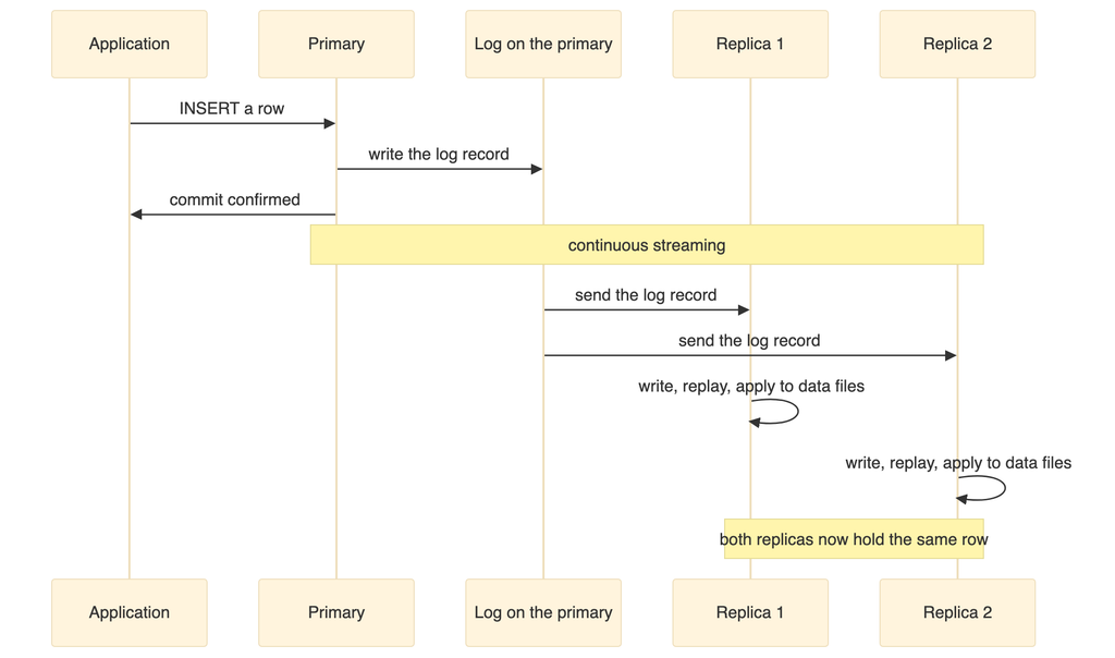
Streaming replication is what keeps the replicas synchronised. It works at the level of the write ahead log, not at the level of SQL statements. A replica receives and replays exactly the same low level changes that the primary made.
This cluster uses asynchronous replication, which the tools report as a synchronisation state of async. That means:
The primary commits a transaction and tells the client it succeeded straight away.
The log records travel to the replicas in the background.
There is a very short window, usually a few milliseconds, in which the primary has committed something the replicas have not received yet.
If the primary is destroyed inside that window, that transaction is lost, because no replica ever saw it.
Synchronous replication is possible and Patroni supports it, but it adds latency to every write, because the primary has to wait for a replica to confirm before it can commit. This lab uses asynchronous replication for simplicity.
The health indicators to watch:
Indicator
Meaning
Healthy value
sent position
How far the primary has sent to this replica
Matches the primary’s current position
write position
How far the replica has written to disk
Matches the sent position
flush position
How far the replica has flushed to disk
Matches the write position
replay position
How far the replica has applied to its data files
Matches the flush position
state
Connection state
The value streaming means healthy
sync state
Synchronisation mode
The value async in this build
When all four positions match, the replication lag is zero.
This setup has real limits, and it is better to be clear about them.
Situation
Protected
Why
One PostgreSQL node fails
Yes
Patroni promotes a replica
Application needs a stable address
Yes
HAProxy provides one
Loss of committed transactions
Mostly
Replicas are very close to real time, but asynchronous replication leaves a tiny window
All nodes fail together
No
Every container runs on one Docker host
etcd fails
No
There is only one etcd node, so no election can happen
Disk corruption
No
Corruption is replicated to the replicas along with everything else
Somebody drops a table by accident
No
The change is replicated to all nodes immediately
Data centre failure
No
Everything is on one machine
Network partition creating two primaries
Partly
The lock in etcd stops two primaries existing, because a leader that loses the lock demotes itself
The important line in that table is the one about dropping a table. Replication is not a backup. Three synchronised copies of a mistake are still a mistake.
PostgreSQL already has table partitioning, where one large table is split into smaller pieces using a declarative partition clause. Partitioning is useful, but every partition still lives on the same PostgreSQL instance, on the same disk, using the same CPU. It does not spread data across machines.
For genuine sharding across nodes, where different rows physically live on different servers, there are three options:
Sharding in the application, so the application decides which database to connect to.
A proxy or middleware layer in front of several databases.
A PostgreSQL extension that handles distribution inside the database.
Citus is the third option. It runs inside PostgreSQL, so you keep standard SQL, standard tools and standard client access, while the data is physically spread across workers.
Capability
PostgreSQL on its own
PostgreSQL with Citus
Store data on more than one server
No
Yes
Route a query to the right shard
No
Yes, automatically
Run one query on many shards in parallel
No
Yes
Join co-located tables without a network hop
Not applicable
Yes
Add or remove nodes while running
Not applicable
Yes
Move data after adding a node
Not applicable
Yes, using logical replication
Standard SQL and tools
Yes
Yes
The honest summary is that partitioning helps you manage a big table on one machine, and sharding helps you use more than one machine. If your problem is that queries scan too much data, partitioning may be enough and is far simpler. If your problem is that one machine is genuinely full, you need sharding.
Two structural points shape everything else in this guide.
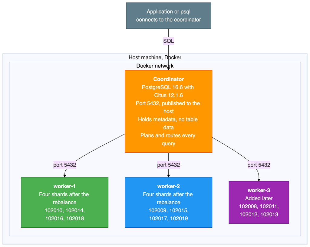
The coordinator stores no table data. It holds only the Citus metadata: which shard lives where, and which range of hash values each shard owns. All 10,500 rows sit on the workers. That makes the coordinator cheap to run, and also makes it a complete single point of failure, as the section on availability explains.
Workers are ordinary, independent PostgreSQL servers. They do not replicate to each other and they are not aware of each other. A shard is a normal PostgreSQL table with a number on the end of its name. You can connect to a worker directly and select from a shard table exactly as you would from any other table.
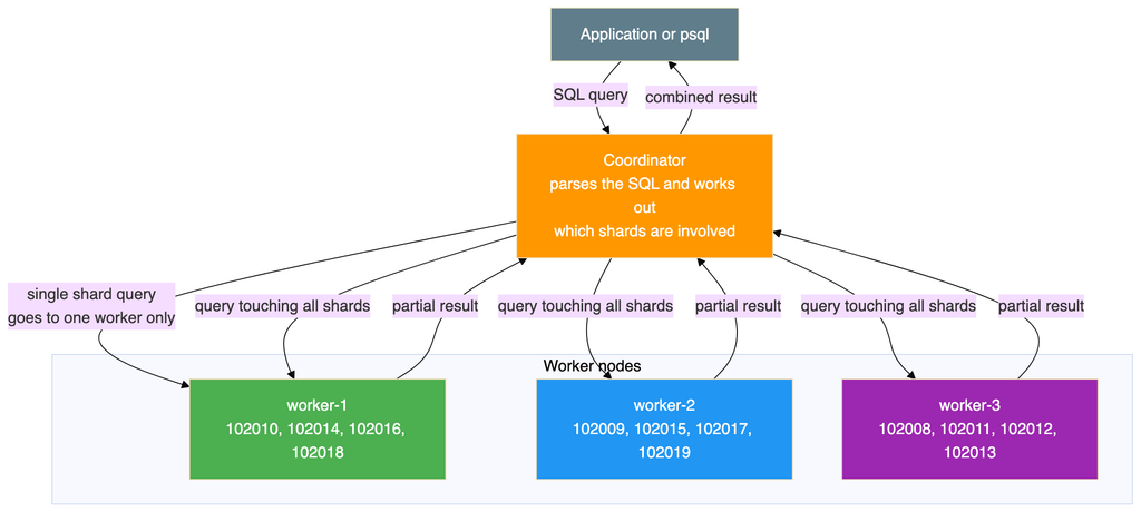
There are two shapes of query here, and the difference matters more than anything else for performance. A query that filters on the shard key goes to exactly one worker. A query that does not filter on the shard key has to be sent to every shard, with each one returning a partial answer for the coordinator to combine.
Citus uses hash based sharding. When a table is distributed on the customer identifier:
Citus hashes the value of that column.
The full range of possible hash values is divided into equal, non overlapping slices, one per shard.
Each shard is placed on a worker.
When a row is inserted, Citus hashes the value, finds which slice it falls into, and sends the row to the worker holding that shard.
When a query filters on that column, the same hash tells the coordinator which single worker to ask.
With twelve shards and three workers, each worker holds four shards. A shard holds a set of customer identifiers that happen to hash into the same slice. It is not a contiguous range of identifiers, which is why customers 100 and 500 can end up on the same shard while 1 and 42 do not.
All three tables are distributed on the same column and placed in the same co-location group. This has three consequences:
Shard number 102008 of the first table sits on the same worker as the matching shards of the other two tables.
A join between those tables on the shared column runs entirely inside one worker, with no data crossing the network.
The rebalancer moves whole co-location groups together, so related rows stay together.
Co-location is the single most consequential design decision in a sharded schema. Get it right and most of your queries touch one node. Get it wrong and almost every query becomes a distributed one, and changing it later means redistributing every table.
The client is optional, because you can run psql inside the coordinator container instead.
The lab runs three or four containers, so give Docker at least 4 GB of memory.
Note: This build was tested on Docker Desktop on Windows, where Linux containers run inside a small virtual machine and all Docker commands work normally from PowerShell. The same files work on macOS and Linux. The one difference is how you feed a SQL file into a container, because piping a file is written differently in PowerShell than in a Unix shell.
There is a small versioning trap here. Citus reports two different version numbers, and they answer different questions. The extension catalogue reports the SQL script version, which is 12.1-1 in this build. The Citus version function reports the compiled library version:
SELECT citus_version();
Which gives the full build string captured in the evidence:
                                     citus_version
----------------------------------------------------------------------------------------
 Citus 12.1.6 on x86_64-pc-linux-gnu, compiled by gcc (Debian 12.2.0-14) 12.2.0, 64-bit
(1 row)
Both numbers are correct. Only the second tells you the patch level, so use that one when you are checking whether a particular fix is present.
The repository holds the Compose file. This section explains what it sets up and why.
Four services sit on one Docker bridge network. The coordinator publishes port 5432 to the host, and the workers do not publish anything, so they are reachable only from inside the network. That mirrors how a real deployment works: clients talk to the coordinator and nothing else.
Each node has its own Docker volume. Every node runs a health check using the standard PostgreSQL readiness tool, every five seconds.
The third worker is defined behind a Compose profile, which means it does not start with the normal start command. It only starts when the profile is named explicitly. That is what makes the add a node exercise realistic, because nothing has to be rebuilt or reconfigured to bring it in.
Citus will not function unless it is loaded at server start
Logical write ahead log level
All nodes
The rebalancer moves shards using logical replication, which requires it
Twelve shards per distributed table
Coordinator
Twelve divides evenly by both two and three workers, which keeps the example tidy
One copy of each shard
Coordinator
No shard level replication in this lab. See the availability section.
Raised background worker limit
All nodes
Citus uses background workers for parallel queries and for rebalancing
Prepared transactions enabled
All nodes
Citus uses two phase commit across workers, which needs these
Trust authentication
All nodes
Passwordless connections inside the Docker network. Suitable for a lab only.
Two of these are worth calling out.
The logical log level and prepared transactions are not optional if you intend to rebalance. Both default to values that make the rebalancer fail, and the failures are not obvious from the error messages. They are the two most common reasons a first attempt at rebalancing does not work.
Trust authentication means no password is required at all. It is convenient in a lab and completely unacceptable anywhere else. Nothing in this build should be exposed to a network you do not fully control.
That loops over the coordinator and both workers, creating the customer_orders database and enabling the Citus extension in each. It has to be done per node, because Citus does not propagate a create database command to the workers.
# PowerShell, which is what the original run used Get-Content scripts/03-create-schema.sql | docker exec -i citus-coordinator psql -U postgres -d customer_orders Get-Content scripts/04-distribute-tables.sql | docker exec -i citus-coordinator psql -U postgres -d customer_orders Get-Content scripts/05-generate-data.sql | docker exec -i citus-coordinator psql -U postgres -d customer_orders
The order matters. The tables have to exist before they can be distributed, and they have to be distributed before the data is loaded, or the rows land on the coordinator instead of the workers.
The first prints the shard placement, the shard count per worker, and the row counts per shard and per worker. The second runs the query plans that show single shard routing and co-located joins.
The script starts the container with its profile, waits for it to accept connections, creates the database and extension on it, registers it with the coordinator, and then prints the shard distribution so you can see that the new worker holds nothing yet.
This prints the distribution before, runs the rebalance synchronously so the shard moves appear as they happen, then prints the distribution, the row counts per worker and the full placement afterwards.
The validation checks the totals, the duplicate counts, referential integrity in both directions, specific customers, the revenue aggregate and the identifier range.
# Open a session on the coordinator
docker exec -it citus-coordinator psql -U postgres -d customer_orders

# Where does every shard live?
docker exec citus-coordinator psql -U postgres -d customer_orders \
  -c "SELECT shardid, shard_name, nodename FROM citus_shards WHERE table_name::text = 'customers' ORDER BY shardid;"

# Which worker owns a given customer?
docker exec citus-coordinator psql -U postgres -d customer_orders \
  -c "SELECT get_shard_id_for_distribution_column('customers', 42);"

# Row count in every shard of a table
docker exec citus-coordinator psql -U postgres -d customer_orders \
  -c "SELECT shardid, result FROM run_command_on_shards('customers', 'SELECT count(*) FROM %s') ORDER BY shardid;"

# Progress of a rebalance that is still running
docker exec citus-coordinator psql -U postgres -d customer_orders \
  -c "SELECT * FROM get_rebalance_progress();"

# Prove a shard is just an ordinary table by reading it on the worker
docker exec citus-worker-1 psql -U postgres -d customer_orders \
  -c "SELECT count(*) FROM customers_102010;"
That last one is the command worth running if sharding still feels abstract. It connects straight to a worker, bypassing Citus entirely, and reads a shard as the plain PostgreSQL table it is.
Starting the stack with the normal Compose command brings up three containers: the coordinator and the first two workers. The third worker stays down, because it sits behind a profile.
Wait until all three report themselves as healthy. This is the container status from the test run:
NAME                IMAGE                  SERVICE       STATUS                  PORTS
citus-coordinator   citusdata/citus:12.1   coordinator   Up 47 hours (healthy)   5432/tcp
citus-worker-1      citusdata/citus:12.1   worker-1      Up 47 hours (healthy)   5432/tcp
citus-worker-2      citusdata/citus:12.1   worker-2      Up 47 hours (healthy)   5432/tcp
The command and creation columns have been left out to fit the page. Wait until all three report healthy.
One detail in that output is worth explaining rather than glossing over. The ports column shows a bare container port for all three, including the coordinator, even though the Compose file publishes the coordinator’s 5432 to the host. The reason is that this column reflects how the running container was actually created, and these containers had been up for 47 hours by the time the snapshot was taken. If you start the cluster from the current Compose file, the coordinator will instead show a published mapping in the form 0.0.0.0:5432->5432/tcp, and the two workers will still show a bare port.
Either way the important point holds: clients connect to the coordinator, and the workers are reachable only from inside the Docker network.
If port 5432 is already in use on your host, which usually means a locally installed PostgreSQL is running, the coordinator will fail to start. Change the published port in the Compose file and connect on the new one.
The Citus image creates the extension automatically in the default database. This lab uses a dedicated database instead, which has to be created on every node, with the extension enabled in each one.
The reason every node needs it is worth understanding. Citus keeps its metadata on the coordinator, but the shards themselves are ordinary PostgreSQL tables on the workers. When the coordinator distributes a table, it sends the schema definition to the workers so they can create the shard tables. If a worker does not have the database and the extension, that step fails.
Note that creating a database is not propagated to the workers automatically in this version, which is why it has to be done on each node. The setup script in the repository does this for all nodes in one pass.
Checking the extension afterwards:
SELECT extname, extversion FROM pg_extension WHERE extname = 'citus';
Result:
 extname | extversion
---------+------------
 citus   | 12.1-1
As noted in the versions section, this is the SQL script version rather than the library version.
The coordinator has to be told which workers exist. It also has to be told its own address, because the rebalancer needs to know about every node in the cluster including the coordinator itself.
-- Tell Citus its own address first
SELECT citus_set_coordinator_host('coordinator', 5432);

-- Then add each worker by hostname and port
SELECT citus_add_node('worker-1', 5432);
SELECT citus_add_node('worker-2', 5432);
The hostnames here are Docker service names, resolved by the container network. On real machines they would be DNS names or addresses the coordinator can reach.
Where to check the node details
This is the query to know, because it is how you confirm the cluster membership at any point:
SELECT nodeid, nodename, nodeport, noderole, isactive
FROM pg_dist_node
ORDER BY nodeid;
pg_dist_node is the Citus metadata table holding one row per node, coordinator included. There is also a helper that returns only the active workers, which is handy in scripts:
SELECT * FROM citus_get_active_worker_nodes() ORDER BY node_name;
After registering the coordinator and the two workers, the node list looked like this:
The role column says primary for every row, and that is a naming collision worth clearing up. This is Citus describing its own internal node classification. It has nothing to do with PostgreSQL streaming replication, and it does not mean these nodes have replicas. Each worker here is completely independent, and there is no replication between them.
Three tables were created. Orders reference customers, and order items reference both.
CREATE TABLE IF NOT EXISTS customers (
    customer_id BIGSERIAL,
    name        TEXT           NOT NULL,
    email       TEXT           NOT NULL,
    city        TEXT           NOT NULL,
    created_at  TIMESTAMPTZ    NOT NULL DEFAULT now(),
    PRIMARY KEY (customer_id)
);

CREATE TABLE IF NOT EXISTS orders (
    order_id     BIGSERIAL,
    customer_id  BIGINT         NOT NULL,
    order_date   DATE           NOT NULL DEFAULT CURRENT_DATE,
    total_amount DECIMAL(10,2)  NOT NULL,
    status       TEXT           NOT NULL DEFAULT 'pending',
    PRIMARY KEY (order_id, customer_id),
    CONSTRAINT fk_orders_customer
        FOREIGN KEY (customer_id) REFERENCES customers (customer_id)
);

CREATE TABLE IF NOT EXISTS order_items (
    item_id      BIGSERIAL,
    order_id     BIGINT         NOT NULL,
    customer_id  BIGINT         NOT NULL,
    product_name TEXT           NOT NULL,
    quantity     INT            NOT NULL,
    unit_price   DECIMAL(10,2)  NOT NULL,
    PRIMARY KEY (item_id, customer_id),
    CONSTRAINT fk_items_customer
        FOREIGN KEY (customer_id) REFERENCES customers (customer_id),
    CONSTRAINT fk_items_order
        FOREIGN KEY (order_id, customer_id) REFERENCES orders (order_id, customer_id)
);
Read the primary keys closely, because they are the part that differs from a normal schema.
There is one design detail that is specific to Citus and that catches everybody the first time.
Every unique constraint has to include the distribution column. The customers table is keyed on the customer identifier alone, which is fine because that is the distribution column. The orders table is keyed on the order identifier together with the customer identifier, rather than the order identifier by itself. The order items table does the same thing.
The reason is that uniqueness can only be enforced inside a single shard. There is no global index spanning all the workers, and building one would require coordination on every insert, which is exactly the cost sharding is meant to avoid. By including the distribution column in the key, Citus knows that all rows which could possibly collide are in the same shard, so a local unique index is sufficient.
The practical consequence is that you cannot simply take an existing schema and distribute it. Primary keys and unique constraints usually have to change first, and foreign keys have to line up with the distribution column too. This is normally the largest piece of work in adopting Citus, and it is worth knowing before you start rather than halfway through.
The shard key for all three tables is the customer identifier. This was a deliberate choice, and the alternatives were considered.
Criterion
Customer identifier
Order identifier
City
Number of distinct values
Good, 500
Good, 2,500
Poor, only 10
Spreads evenly
Yes, hashing distributes it
Yes
No, 50 customers per city
Allows co-located joins
Yes, all three tables have it
No, the customers table does not have it
No, the other tables do not have it
Commonly used as a filter
Yes, show me this customer’s data
Sometimes
Sometimes
Keeps one customer’s data together
Yes
No
No
The customer identifier wins for four reasons:
It exists in all three tables, so a customer, their orders and their order items all land on the same shard.
Joins on it stay local, with no data moving between workers.
A lookup for one customer touches one worker, not all of them.
It spreads reasonably evenly. Hashing 500 identifiers across twelve shards averages about 42 per shard. The observed spread was 32 to 47, which is normal variation at this size and evens out with more data.
What a bad shard key looks like. If the city column had been used, all 50 customers in one city would sit on a single shard. With only ten distinct cities and twelve shards, at least two shards would be permanently empty while the others carried everything. Worse, the imbalance would be invisible in a small test and would only become a problem at scale.
The general rule is that a good shard key has many distinct values, spreads them evenly, appears in most of your queries as a filter, and exists in all the tables you want to join. A tenant or customer identifier usually fits. A status column, a boolean, a country, or anything with a handful of values does not.
The tables were created as ordinary PostgreSQL tables first, then converted into distributed tables, with the second and third explicitly co-located with the first.
The colocate_with argument is the important one, and leaving it out is the most consequential mistake you can make here. Without it Citus is free to put each table in its own co-location group, and a join between them stops being local. It is worth being explicit even when Citus would have guessed correctly, because the intent is then recorded in the schema rather than left to a default.
The distribution was then confirmed with:
SELECT logicalrelid::text AS table_name,
       partmethod,
       colocationid,
       repmodel
FROM pg_dist_partition
ORDER BY logicalrelid::text;
What that conversion does:
Creates twelve shard tables on the workers, named after the original table with a shard number appended.
Gives each shard an equal, non overlapping slice of the hash space, recorded in the Citus metadata.
Assigns shards to workers in turn, in shard number order. With two workers that produced a strict alternation: the first shard to worker 1, the second to worker 2, the third to worker 1, and so on.
Places the co-located tables’ shards on the same workers as the matching shards of the first table.
Confirming the result:
 table_name  | partmethod | colocationid | repmodel
-------------+------------+--------------+----------
 customers   | h          |            1 | s
 order_items | h          |            1 | s
 orders      | h          |            1 | s
The partition method is hash. All three tables share co-location group 1, which is what makes local joins possible. The replication model column reports the streaming model, meaning a single copy of each shard.
Citus allocates shard numbers from one counter, in a contiguous block per table, in the order the tables were distributed.
Table
Shard numbers
Distributed
customers
102008 to 102019
First
orders
102020 to 102031
Second
order_items
102032 to 102043
Third
Co-located shards line up by position within the block, not by having the same number. The first customers shard is co-located with the first orders shard and the first order items shard. This is why a later section shows shard 102008 moving together with 102020 and 102032. They are one co-location group covering the same slice of the hash space, and Citus always moves them as a unit.
It also explains a number that would otherwise look arbitrary. The eleventh customers shard, 102018, pairs with the eleventh orders shard, 102030, which is the pairing the co-located join example relies on.
The data was generated entirely in SQL, using generate_series and cross joins rather than a loop:
-- 500 customers, cities cycling through a list of ten
INSERT INTO customers (name, email, city)
SELECT
    'Customer-' || i,
    'customer' || i || '@example.com',
    (ARRAY['New York', 'London', 'Tokyo', 'Paris', 'Sydney',
           'Berlin', 'Toronto', 'Mumbai', 'São Paulo', 'Singapore'])[1 + (i % 10)]
FROM generate_series(1, 500) AS s(i);

-- 5 orders for every customer, so 2,500 rows
INSERT INTO orders (customer_id, order_date, total_amount, status)
SELECT
    c.customer_id,
    CURRENT_DATE - (floor(random() * 365))::int,
    round((random() * 490 + 10)::numeric, 2),
    (ARRAY['pending', 'shipped', 'delivered', 'cancelled'])[1 + floor(random() * 4)::int]
FROM customers c
CROSS JOIN generate_series(1, 5) AS s(n);

-- 3 items for every order, so 7,500 rows
INSERT INTO order_items (order_id, customer_id, product_name, quantity, unit_price)
SELECT
    o.order_id,
    o.customer_id,
    (ARRAY['Widget', 'Gadget', 'Gizmo', 'Doohickey',
           'Thingamajig', 'Sprocket', 'Flange', 'Bracket'])[1 + floor(random() * 8)::int],
    1 + floor(random() * 10)::int,
    round((random() * 99 + 1)::numeric, 2)
FROM orders o
CROSS JOIN generate_series(1, 3) AS s(n);
Two things follow from how this is written. The city assignment uses the row number modulo ten, which is why every city ends up with exactly fifty customers rather than an approximate share. The amounts and dates use random(), which is why the revenue figures shown later cannot be reproduced on your machine even though the row counts can.
Table
Rows
How
customers
500
One per generated number
orders
2,500
Five per customer
order_items
7,500
Three per order
Total
10,500
Every insert went through the coordinator. The coordinator hashed each row’s customer identifier and sent the row to the correct worker, with no involvement from the client. This is the part that makes Citus pleasant to use: the application inserts rows as if into a normal table.
The script finishes by counting what it loaded:
SELECT 'customers'   AS table_name, count(*) AS row_count FROM customers
UNION ALL SELECT 'orders',      count(*) FROM orders
UNION ALL SELECT 'order_items', count(*) FROM order_items
ORDER BY table_name;
This is where sharding stops being abstract. The citus_shards view is the one to know: it lists every shard, which table it belongs to, which node holds it and how large it is.
SELECT shardid, shard_name, table_name::text, nodename, nodeport, shard_size
FROM citus_shards
WHERE table_name::text = 'customers'
ORDER BY shardid;
The shard placement for the customers table, before the third worker was added:
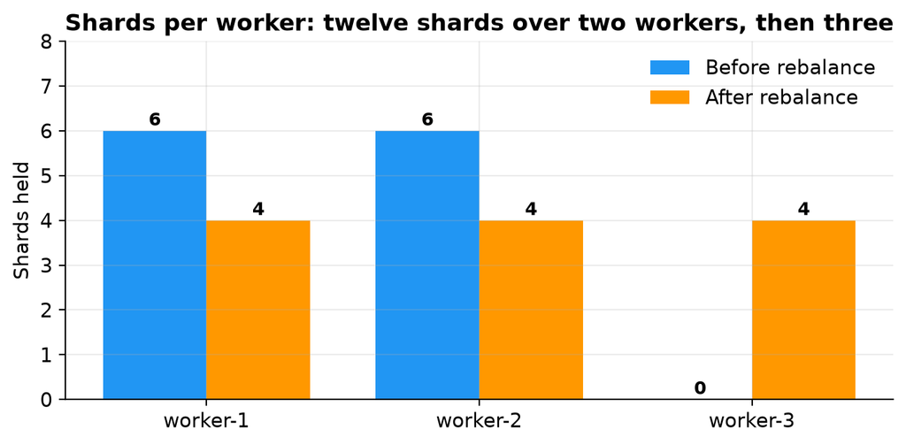
Twelve shards alternating between the two workers, six each. Every one is a real PostgreSQL table sitting in a worker’s database.
Row counts per worker. This one needs run_command_on_shards, which sends the same SQL to every shard of a table and returns the results as rows, with %s standing in for the shard’s real table name:
SELECT cs.nodename,
       count(*)              AS shard_count,
       sum(r.result::bigint) AS total_rows
FROM run_command_on_shards('customers', $cmd$ SELECT count(*) FROM %s $cmd$) r
JOIN citus_shards cs USING (shardid)
WHERE cs.table_name::text = 'customers'
GROUP BY cs.nodename
ORDER BY cs.nodename;
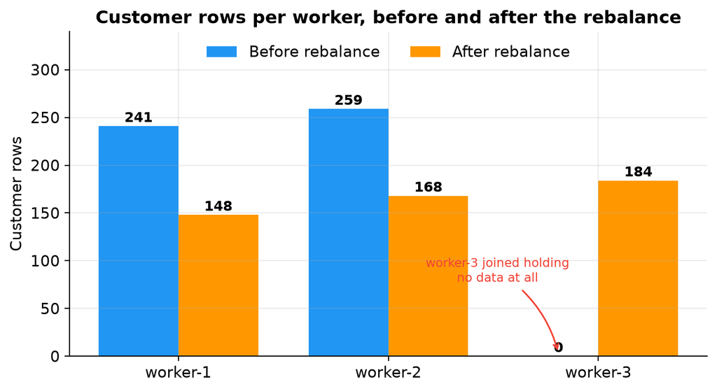
That totals 500. The small imbalance between 241 and 259 is expected, because hashing distributes values approximately rather than exactly.
The same ratio appears in all three tables, because they are co-located:
Table
worker-1
worker-2
Total
customers
241
259
500
orders
1,205
1,295
2,500
order_items
3,615
3,885
7,500
A customer with five orders and fifteen order items always lands on one worker, so the proportions follow the customer distribution exactly.
Row counts per individual shard, using the same function without the grouping:
SELECT shardid, success, result AS row_count
FROM run_command_on_shards('customers', $cmd$ SELECT count(*) FROM %s $cmd$)
ORDER BY shardid;
Result:
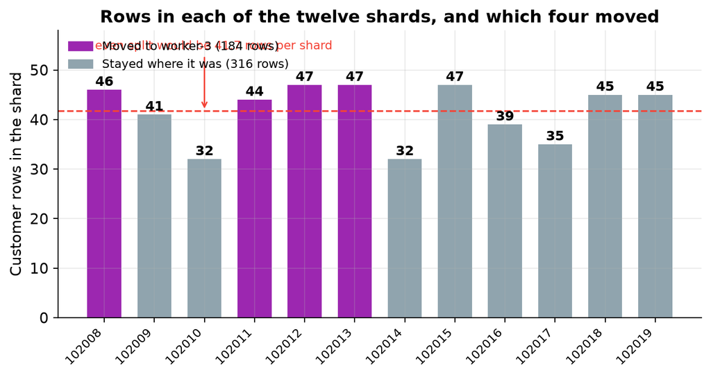
 shardid | success | row_count
---------+---------+-----------
  102008 | t       | 46
  102009 | t       | 41
  102010 | t       | 32
  102011 | t       | 44
  102012 | t       | 47
  102013 | t       | 47
  102014 | t       | 32
  102015 | t       | 47
  102016 | t       | 39
  102017 | t       | 35
  102018 | t       | 45
  102019 | t       | 45
The range is 32 to 47 rows. The variation comes from the hash function, because some slices catch more identifiers than others. With more data the distribution evens out. These twelve numbers are used later to prove that the rebalance did not lose anything.
The chart makes two things visible at once. The bars show how uneven hash distribution really is at this scale: the busiest shard holds 47 rows and the quietest 32, against an even split of 41.7. Nothing is wrong, and no amount of tuning would flatten it, because the hash function is doing its job of scattering values rather than balancing counts.
The four coloured bars are the shards that the rebalancer later moved. Notice that it did not pick the four largest or the four smallest. It picked the set that produced an even shard count, which is a different objective, and the 184 rows that ended up on worker-3 are simply the consequence of that choice.
EXPLAIN (VERBOSE) SELECT * FROM customers WHERE customer_id = 42;
Asking for one customer by identifier produced a plan with a task count of one, naming a single shard and a single worker. Citus worked out that the identifier hashes to shard 102018, which was on worker 1, and sent the query only there. The other worker was not contacted at all.
This is the best case, and it is the case worth designing for. Adding more workers makes this kind of query no slower, because it always touches exactly one of them.
SELECT c.name, o.order_id, o.order_date, o.total_amount, o.status
FROM customers c
JOIN orders o ON c.customer_id = o.customer_id
WHERE c.customer_id = 42
ORDER BY o.order_date;
Joining customers to orders for one customer also produced a task count of one. Both tables’ shards for that customer are on the same worker, so the whole join ran there. No data moved between workers.
SELECT c.city,
       count(DISTINCT c.customer_id) AS customers,
       count(o.order_id)             AS orders,
       round(sum(o.total_amount), 2) AS total_revenue
FROM customers c
JOIN orders o ON c.customer_id = o.customer_id
GROUP BY c.city
ORDER BY total_revenue DESC;
Grouping revenue by city has no filter on the shard key, so it has to touch every shard. Each worker computed a partial result and the coordinator combined them:
   city    | customers | orders | total_revenue
-----------+-----------+--------+---------------
 Sydney    |        50 |    250 |      66162.73
 Toronto   |        50 |    250 |      65014.76
 Berlin    |        50 |    250 |      64942.73
 Paris     |        50 |    250 |      64364.26
 São Paulo |        50 |    250 |      63762.02
 Singapore |        50 |    250 |      63306.32
 Tokyo     |        50 |    250 |      62648.80
 New York  |        50 |    250 |      62305.02
 Mumbai    |        50 |    250 |      61182.11
 London    |        50 |    250 |      58398.65
Fifty customers in every city, totalling 500, which confirms nothing was missed. This query runs on all shards in parallel, so it is not slow, but it does get more expensive as workers are added rather than less. That is the trade-off of a query that cannot be routed to one shard.
Note the exactly even fifty per city. That is an artefact of how the sample data was generated, not a property of the hashing.
Asking Citus directly which shard a given identifier belongs to:
SELECT 1::bigint AS customer_id, get_shard_id_for_distribution_column('customers', 1) AS shard_id
UNION ALL SELECT 42,  get_shard_id_for_distribution_column('customers', 42)
UNION ALL SELECT 100, get_shard_id_for_distribution_column('customers', 100)
UNION ALL SELECT 250, get_shard_id_for_distribution_column('customers', 250)
UNION ALL SELECT 500, get_shard_id_for_distribution_column('customers', 500);
Identifiers 100 and 500 both map to shard 102014, while 1 and 42 are on different shards. This is what hash distribution means in practice. Shards hold sets of identifiers that hash together, not contiguous ranges, so you cannot look at a shard and describe its contents as a range.
The approach. Rather than starting with three workers, the cluster was deliberately built with two, filled with data, and only then extended. That is the situation people actually face, and it is the one where the interesting question arises, because the existing data has to move.
What was captured, and when. A full snapshot of the cluster state was written to files at two points: after the third worker was registered but before any rebalance, and again after the rebalance finished. Each snapshot recorded the container status, the Citus version, the node list, the shard placement, the shard count per worker, the row counts per worker for all three tables, the total row counts, and a sample of rows. The before and after tables later in this document are built from those two snapshots.
What was checked afterwards. Row totals for all three tables, duplicate checks on the keys, referential integrity in both directions, spot checks on specific customers, the revenue aggregate compared against its pre-rebalance value, and the range of customer identifiers.
What would have counted as a failure. Any change in a row total, any duplicate, any orphan row, or any difference in the revenue figures. None of those occurred.
The scripts that add the worker, run the rebalance, capture the snapshots and validate the data are in the repository.
The third worker was started using its Compose profile. Only that container started, and the coordinator and existing workers kept running without interruption.
Then the same preparation as any other worker: wait for it to be healthy, create the database, enable the extension, and register it with the coordinator.
The node list afterwards, from the same pg_dist_node query as before:
SELECT nodeid, nodename, nodeport, noderole, isactive
FROM pg_dist_node
ORDER BY nodeid;
The new worker holds nothing. It does not even appear in the list, because it owns no shards. Adding a node to Citus registers it and nothing more. The existing shards stay exactly where they were.
This is deliberate, and it is the right default. Moving data costs disk reads, network transfer and write ahead log volume on the source workers. Citus separates the decision that a node exists from the decision to pay that cost, so you can add capacity during a quiet period and move data during a quieter one. New distributed tables created from this point would use the new worker straight away, but existing data waits until you ask.
NOTICE: Moving shard 102011 from worker-2:5432 to worker-3:5432 … NOTICE: Moving shard 102008 from worker-1:5432 to worker-3:5432 … NOTICE: Moving shard 102013 from worker-2:5432 to worker-3:5432 … NOTICE: Moving shard 102012 from worker-1:5432 to worker-3:5432 …
Four shard groups moved: two from the first worker and two from the second. Each of those moves carried the co-located shards from all three tables, so moving shard 102008 also moved the matching orders and order items shards.
Those notices came from the interactive session rather than the evidence snapshots, but the captured placement afterwards confirms the same four moves independently:
SELECT shardid, shard_name, nodename FROM citus_shards WHERE table_name::text = 'customers' ORDER BY shardid;
Comparing this against the placement captured before the rebalance, the four shards now on worker-3 are exactly 102008, 102011, 102012 and 102013, and the remaining eight have not moved. The notices and the snapshot agree.
Notice what the rebalancer chose to do. It moved four shard groups, not twelve. It worked out the smallest set of moves that produces an even spread, and left the other eight groups untouched. That restraint matters on a real cluster, where moving a shard is expensive.
The distribution afterwards:
SELECT nodename, count(*) AS shard_count
FROM citus_shards
WHERE table_name::text = 'customers'
GROUP BY nodename
ORDER BY nodename;
Twelve shards across three workers, four each. The container list at this point, remembering that the profile has to be named or the third worker is left out:
docker compose –profile add-shard ps
It shows the newcomer alongside the original three, having been running for 43 minutes against their two days:
NAME                IMAGE                  SERVICE       STATUS
citus-coordinator   citusdata/citus:12.1   coordinator   Up 2 days (healthy)
citus-worker-1      citusdata/citus:12.1   worker-1      Up 2 days (healthy)
citus-worker-2      citusdata/citus:12.1   worker-2      Up 2 days (healthy)
citus-worker-3      citusdata/citus:12.1   worker-3      Up 43 minutes (healthy)
That uptime difference is the point of the exercise. The three original containers were never restarted, never reconfigured and never taken offline. Capacity was added and data was moved onto it while they carried on serving.
Row counts afterwards:
SELECT cs.nodename,
       count(*)              AS shard_count,
       sum(r.result::bigint) AS total_rows
FROM run_command_on_shards('customers', $cmd$ SELECT count(*) FROM %s $cmd$) r
JOIN citus_shards cs USING (shardid)
WHERE cs.table_name::text = 'customers'
GROUP BY cs.nodename
ORDER BY cs.nodename;
Note that the row counts are less even than the shard counts. Four shards each, but 148, 168 and 184 rows.
That is expected, because the rebalancer does not look at row counts at all. Citus assigns every shard a cost and then equalises the total cost per worker. In version 12.1 the default strategy is by_disk_size, which uses the shard’s size on disk as its cost. An older strategy called by_shard_count gives every shard a cost of 1, which makes balancing the cost the same as balancing the number of shards. You can switch between them, or define your own.
In this lab the two strategies would produce the same plan, because the data is small and every shard reported the same size on disk. That is why the result came out as a clean four, four and four. On a real cluster with shards of genuinely different sizes the two strategies diverge, and you can end up with an uneven shard count precisely because the sizes were being equalised instead.
Either way, an even shard count does not imply an even row count, and neither is what the rebalancer is aiming for.
Four of twelve shards moved, two from each existing worker.
Shard count per worker:
Worker
Before
After
Change
worker-1
6
4
Two fewer
worker-2
6
4
Two fewer
worker-3
0
4
Four more
Row count per worker for the customers table:
Worker
Before
After
Change
worker-1
241
148
93 fewer
worker-2
259
168
91 fewer
worker-3
0
184
184 more
Total
500
500
No change
This is the chart that shows what a rebalance actually is. The two original workers each gave up roughly a third of their rows, the new worker went from nothing to 184, and the total stayed at 500. No row was created and none was lost. The load simply moved.
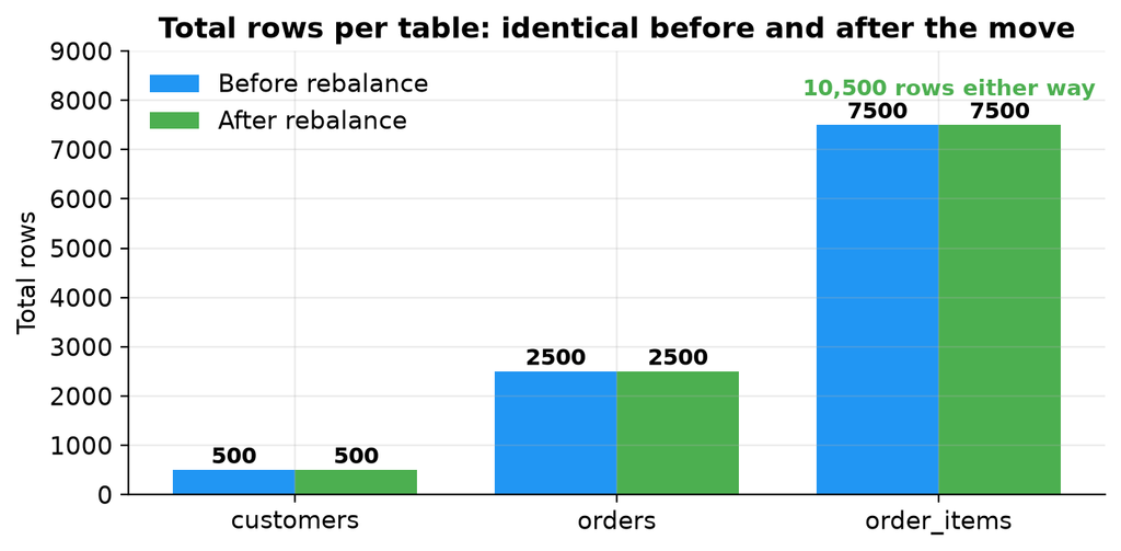
Total row counts:
Table
Before
After
customers
500
500
orders
2,500
2,500
order_items
7,500
7,500
Total
10,500
10,500
A chart of two identical sets of bars is a dull picture, and that is the entire point. Physically relocating a third of the data across the network changed nothing that the application can observe.
The per shard counts from the earlier section reconcile exactly against the per worker totals, which is the strongest evidence available that nothing was lost or duplicated.
Worker
Shards held
Row counts
Total
worker-1, before
102008, 102010, 102012, 102014, 102016, 102018
46, 32, 47, 32, 39, 45
241
worker-2, before
102009, 102011, 102013, 102015, 102017, 102019
41, 44, 47, 47, 35, 45
259
worker-1, after
102010, 102014, 102016, 102018
32, 32, 39, 45
148
worker-2, after
102009, 102015, 102017, 102019
41, 47, 35, 45
168
worker-3, after
102008, 102011, 102012, 102013
46, 44, 47, 47
184
Both groupings total 500, and every shard arrived holding exactly the rows it started with.
That last point is the important one. A shard move relocates data. It does not re-hash it. The distribution column decides which shard a row belongs to, and that never changed. Only the shard’s location changed. This is why a rebalance is safe to run on a live cluster: Citus is not recalculating anything, so there is no moment when a row could belong to two shards or to none.
The validation script was run after the rebalance. These are the checks that matter, and they are worth running on any cluster after a shard move rather than trusting the shard counts alone.
-- Totals must match what was loaded
SELECT 'customers' AS table_name, count(*) AS total FROM customers
UNION ALL SELECT 'orders',      count(*) FROM orders
UNION ALL SELECT 'order_items', count(*) FROM order_items
ORDER BY table_name;

-- A shard copied twice would show up here
SELECT count(*) AS duplicate_customers
FROM (SELECT customer_id FROM customers
      GROUP BY customer_id HAVING count(*) > 1) dupes;

-- A half moved co-location group would break this
SELECT count(*) AS orphan_orders
FROM orders o
LEFT JOIN customers c ON o.customer_id = c.customer_id
WHERE c.customer_id IS NULL;

SELECT count(*) AS orphan_items
FROM order_items oi
LEFT JOIN orders o ON oi.order_id = o.order_id AND oi.customer_id = o.customer_id
WHERE o.order_id IS NULL;

-- Range should still be the full 1 to 500
SELECT min(customer_id) AS min_id, max(customer_id) AS max_id FROM customers;
The two orphan checks are the ones that would actually catch a botched rebalance. If Citus had moved a customers shard without its matching orders shard, those joins would start finding rows with no partner and the counts would stop being zero.
Check
Expected
Actual
Result
Total customers
500
500
Passed
Total orders
2,500
2,500
Passed
Total order items
7,500
7,500
Passed
Duplicate customer identifiers
0
0
Passed
Duplicate orders
0
0
Passed
Orders with no matching customer
0
0
Passed
Order items with no matching order
0
0
Passed
Order count for a specific customer
5
5
Passed
Another customer, five orders and fifteen items
Yes
Yes
Passed
Revenue by city matches the pre-rebalance figures
Yes
Yes
Passed
Range of customer identifiers
1 to 500
1 to 500
Passed
Co-located joins, three table joins and aggregate queries all returned the same results as before the rebalance.
The referential integrity checks are the ones worth noting. Because the tables are co-located, a customer and their orders moved together. If the rebalancer had moved them independently, a join would have started returning rows with no match, and the orphan checks would have caught it. They returned zero.
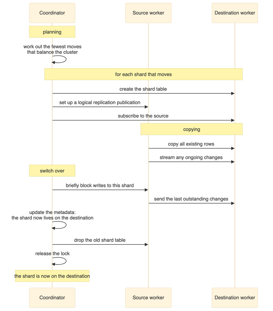
The shard stays readable while it is being copied. Queries continue to work and are served by the source worker until the switch over happens.
The copy uses logical replication. This is why the logical log level is required on every node. Citus creates a temporary publication and subscription, copies the data, then removes them.
The switch over is brief but it is not free. Citus locks the shard, waits for replication to catch up, updates the metadata, drops the old copy and releases the lock. For small shards this takes milliseconds. For large shards under write load it takes longer, and writes to that one shard wait during it. Other shards are unaffected.
Co-located shards move as a group, which is what keeps related rows together and keeps joins local.
The coordinator metadata is the authority. Once the move is recorded, any query hashing to that shard is routed to the new worker.
The shards on that worker are unavailable. With a single copy of each shard there is no replica, so queries needing those shards fail.
The coordinator fails
Everything fails. It is the only entry point.
A worker fails during a rebalance
The rebalance stops. The shard stays on the source worker, and no data is lost.
The coordinator fails during a rebalance
Incomplete moves are cleaned up, because Citus records the state of each move in its metadata. Leftover tables from an interrupted move can be removed with the Citus cleanup function.
This is the part of the guide worth pausing on, because it runs against the intuition that more machines means more resilience.
As built, this cluster is less available than a single PostgreSQL server. With one copy of each shard and four containers, there is no redundant copy of anything, and any one of those four failing takes down some or all of the database. The number of things that can break has been multiplied by four and no redundancy has been added.
Sharding is a technique for scale, not for availability. Treating the two as the same thing is a genuinely dangerous mistake, and it is an easy one to make because both are described as distributing the database.
Citus does have a setting for more than one copy of each shard, but it is not the answer here. That mechanism is statement based replication intended for append only workloads, it is deprecated in current Citus, and it does not apply to the hash distributed tables used in this lab.
More shards give finer control when rebalancing, but add overhead to every query that touches all of them. The Citus default is 32. This lab uses 12 to keep the output readable.
Distinct values in the shard key
Too few values creates hotspots. Five hundred customer identifiers work well. A boolean would be a terrible choice.
Co-located joins
Joins on the shard key run inside one worker with no network cost. Joins on other columns require moving data between workers, which is far more expensive.
Network latency
Everything here is on one host. In a real deployment the latency between nodes affects every query that touches more than one shard.
Rebalancing under load
The rebalancer adds write ahead log volume and disk activity on the source worker. Schedule it for a quiet period.
The single largest performance factor is not in this table. It is whether your queries filter on the shard key. A query that does touches one worker. A query that does not touches all of them, and no amount of tuning changes that.
Adding a worker. Always the same sequence: start it, create the database and the extension, register it with the coordinator, then rebalance when you are ready to move data.
Removing a worker. Drain it first, which moves its shards elsewhere, and only then remove it. Removing a worker that still holds shards loses data.
Monitoring the distribution. The Citus shards view shows where every shard lives and how large it is. Grouping it by table and node gives you the balance at a glance. It is worth checking after every rebalance and occasionally in between, because shards grow at different rates.
Watching a rebalance in progress. Citus provides a progress function that reports how far each shard move has got. This is more useful than it sounds on a large cluster, where a rebalance can run for a long time.
Counting rows per shard. Citus can run the same command on every shard of a table and return the results together, which is how the per shard counts in this document were produced. It is the quickest way to spot a skewed distribution.
The exact queries and functions are in the repository scripts.
Patroni and streaming replication for the coordinator
All containers on one host
No real network separation, and one machine to lose
Separate physical or virtual machines
Trust authentication
No security at all
TLS with password or certificate authentication
No backups
Data loss is permanent
Base backups and log archiving on every node, with restores tested
No monitoring
Problems are invisible until they are serious
Metrics collection and query statistics
One copy of each shard
No redundancy
Each worker behind its own highly available cluster
Twelve shards
Too few to spread across a larger cluster later
Between 32 and 128, depending on how large you expect to grow
No connection pooling
Connection overhead on the coordinator
A connection pooler in front of the coordinator
The shard count deserves a note. Choosing it is more consequential than it looks, because changing it later means redistributing every table. Pick a number with plenty of factors, comfortably larger than the number of workers you expect, so that future rebalances can spread evenly.
The first attempt called a function that does not exist, and PostgreSQL reported that no such function was available.
The name used was a plausible looking blend of two real ones. Citus exposes two different ways to start a rebalance:
Function
Behaviour
The synchronous rebalance function
Blocks the session until every shard has moved, printing each move as it happens. This is what produced the output shown earlier. It is formally deprecated as of Citus 11.2, but still works in 12.1.6.
The background rebalance function
The supported replacement. Schedules the work as a background job and returns immediately. Separate functions report its status, wait for it, and stop it.
The synchronous form was used here on purpose, because printing each move is what makes the mechanism visible. For production use the background form. The deprecation is not arbitrary: a real rebalance can run for hours, and a synchronous call ties its fate to whoever happened to be logged in.
The rebalancer refused to start, reporting that prepared transactions need to be enabled.
The cause is that the relevant PostgreSQL setting defaults to zero, while Citus uses two phase commit across workers during a shard move. The fix is to raise it in the server settings on every node, which the Compose file in the repository now does.
Shard moves failed because the write ahead log level was not set to logical.
The rebalancer copies data using logical replication, so that level is required on every node, not just the coordinator. This is set in the Compose file for all services.
The cause was either that the container was not ready yet, or that the database did not exist on it. The fix is to wait for the readiness check to pass, then create the database and the extension, and only then register the node.
A query calling a function to find which shard owns a value failed, because the name was slightly wrong. The correct name refers to the distribution column rather than the distribution value. This is easy to get wrong from memory, and the error message names the function that was not found, which makes it quick to spot.
Stopping the cluster with the normal Compose command, including the profile so the third worker is included, removes the containers but keeps the named volumes, so starting again brings the data back.
Adding the volume removal flag deletes all four volumes and every row with them. The next start builds an empty cluster.
Remember to include the profile in the shutdown command. Without it the third worker is not part of the operation and its container and volume are left behind, which is confusing the next time you start up.
Phase 1, the initial cluster. Three containers: coordinator, worker 1 and worker 2. Twelve shards per table, six on each worker. Data loaded: 500 customers, 2,500 orders and 7,500 order items. Customer rows split 241 and 259. All queries working.
Phase 2, the third worker added. Four containers. Shards still six and six, with zero on the new worker. The new worker was registered and active but held no data, which is the expected behaviour.
Phase 3, after the rebalance. Four shard groups moved to the new worker: 102008, 102011, 102012 and 102013. Shards evenly split four, four and four. Customer rows split 148, 168 and 184. Total rows unchanged at 10,500. No duplicates, no orphan rows. Joins and aggregates returned identical results.
Adding a node does nothing until you rebalance. The third worker joined and sat empty. Citus keeps the decision that a node exists separate from the decision to move data onto it, so you control when the cost is paid.
Co-location is the decision you cannot cheaply undo. Distributing all three tables on the same column is why joins stayed on one worker and why the rebalancer could move related rows as a unit. Getting it wrong makes almost every query distributed, and fixing it later means redistributing everything.
The shard key has permanent consequences. It decides which queries are fast, which have to touch every node, and where hotspots form. The city column would have looked acceptable in a small test and failed at scale.
A rebalance moves shards, it does not re-hash rows. Every shard arrived holding exactly the rows it left with. That property is what makes an online rebalance trustworthy.
Sharding is not high availability. With one copy of each shard, this cluster has four single points of failure. Scale and resilience are different problems and need different solutions.
Sharding has permanent costs. Queries that do not filter on the shard key get slower. Unique constraints have to include the distribution column, which usually means changing your schema. Foreign keys are constrained. Every operational task multiplies by the number of nodes.
Before reaching for it, exhaust the cheaper options: better indexing, query tuning, connection pooling, read replicas, table partitioning, and simply using a larger machine. Modern hardware runs single node PostgreSQL databases into the multi terabyte range without complaint.
Shard when you have a demonstrated limit on write throughput or data volume that one machine genuinely cannot meet, and when your access patterns have a natural distribution key, usually a tenant or customer. If you cannot name that key with confidence, you are not ready to shard.
Deliberately choose a bad shard key on a copy of this schema, load the same data, and watch the skew appear in the per shard counts.
Add a reference table, which is a small lookup table copied to every worker, and see how it turns previously distributed joins into local ones.
Drain a worker and remove it, then confirm the row counts still reconcile.
Combine this lab with the Patroni guide in the same repository: put each worker behind its own highly available cluster, then stop a worker’s primary while a query is running.
The sharding build is in the postgres-sharding-lab folder. This document explains what each step does and what happened when it was tested. It does not reproduce the files themselves, so please read them in the repository if you plan to adapt them.